Author: Aidan Burrell
Peer reviewers: Chris Nickson, Dash Gantner
Nuts and Bolts of EBM Part 5
You are discussing a theory you have with a colleague – that drinking coffee makes you happier. Your friend however disagrees….
You therefore decide to study this question further. You begin by surveying all the doctors in your hospital, asking them if they drink coffee and how happy they are, as well as subjecting them to a battery of “happiness” tests, to figure out their “mean happiness scores”.
Q1. Describe the null hypothesis and alternative hypothesis for this study.
The null hypothesis is that the mean happiness score of those that drink coffee is NOT different than those that do drink coffee.
The alternative hypothesis is that the mean happiness score of those that drink coffee IS different than those that do drink coffee. You can also say that the data are NOT consistent with the null hypothesis.
Note: Hypothesis testing terminology can get a little confusing – why do we start with null (no difference) hypothesis? The reason is it is easier to disprove an assertion than to prove that it is true. Note also, that even if the data are consistent with a hypothesis, it doesn’t necessarily prove that the alternative is true.
A total of 125 doctors fill complete your study – 75 drink coffee and 50 poor lost souls don’t. The happiness scale goes from 0 (really sad) to 100 (maximally happy).
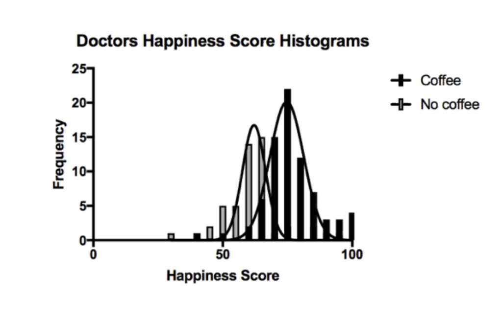
Q2. Describe what type of data is in the graph above, and what is the likely distribution?
The graph above (a frequency distribution) shows the happiness score of those doctors that don’t drink coffee (grey) and those that do (black). These quantitative data are potentially continuous variables if they can take any value from 0-100 (e.g. 59.637). However, they could also be discrete values if the data can only take specific values (e.g. integers). This would depend on how the happiness score is obtained. Let us assume that the data is continuous.
The data has a normal distribution. Normally distributed data is bell shaped, with two roughly equal tails on either side. The central part of the bell correlates with the mean – which is the sum of all values divided by the total number of observations.
Parametric tests can be used on this data as the distribution is known. Otherwise we would need to use non-parametric tests, which make no assumptions about the probability distribution of the data being analysed.
Q3. In the graph above, you notice much variation across the two frequency distributions. What are the causes of variation in this data?
The differences may be real differences between the two populations – coffee drinking populations and non coffee drinking populations.
- Biological differences (eg genes, gender, age, race etc)
They may also be a result of errors, which include:
- Differences in conditions of measurement (non standardized conditions such as different time of day, verbal vs face to face etc)
- Errors of measurement (missing data, incorrectly recorded etc)
- Random variation
The different types of error shown below:
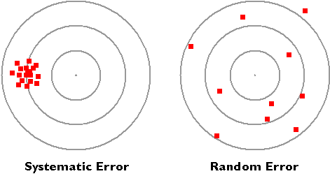
Systematic errors versus random errors. Source: https://www.e-education.psu.edu/natureofgeoinfo/c5_p5.html (Click image for source)
The centre of the target represents the true result. Variation away from the bulls eye in one direction (left) is called systematic error, and this introduces bias. Variation that is random and all over the place (right) doesn’t introduce bias but random error. Both have the effect of reducing the accuracy and certainty of your data.
Statistics can account for random error, but cannot fix systematic bias.
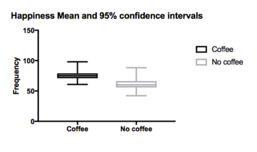
The mean happiness scores and 95% confidence intervals for coffee drinkers vs non coffee drinks are 76 (74-78) vs 61 (58-64). This gives a mean difference of 14 (11-18).
Q4. What do these 95% confidence intervals mean?
A 95% confidence interval is often thought of as the interval in which there is a 95% probability that the true result will lie within. This is a useful subjective approximation but isn’t strictly true. In reality, what it means is that if infinitely repeated samples were taken and the 95% confidence interval was computed for each, then 95% of the confidence intervals would contain the true population value.
Confidence intervals are helpful when you know the mean of your sample, but do not know the true mean of the total population (in this example, it would be all doctors who drink coffee – not just the 150 in the study). What we would really like to know is the mean of the whole population, but we can only know the mean of our sample, so confidence intervals are useful as they give us a range of possible means that the true population mean most likely lies within.
The difference of means between the coffee drinkers and non drinkers reflects the interval of values where the true difference lies – in this case 11-18. As this difference does not contain 0, it indicates that there is a statistically significant difference between the populations.
A narrower range reflects a higher degree of certainty. This can be achieved by increasing sample size, or increasing the precision of the measurements to reduce variability.
Next you want to test your hypotheses that the two groups are truly different. Using your statistical chart, you identify the student T test as the appropriate test to perform (comparing two means from independent groups that are normally distributed). You put this into a stats program and you get a P-value of <0.001.
Q5. What does this P-value mean?
The P-value is the probability or likelihood that a difference observed (or one more extreme) might have occurred by chance, if the null hypothesis is true. The smaller the P-value, the greater the evidence against the null hypothesis. It helps us distinguish explained differences (ie a true difference) from unexplained variation (random error or chance).
In our example, the mean happiness score of non coffee drinkers is 61 compared with coffee drinkers at 76. The T test gives us a probability that this result is due to chance (or false positive rate) of P=<0.001. This means there is a less than 0.1% chance it was due chance, and a 99.9% change it was a real difference.
By convention, a P-value of <0.05 is an agreed and acceptable false positive rate for clinical studies. This means that 95% or 19/20 results that show a difference will be a true difference. For an analogy with the courts, to convict a criminal, the jury must find the criminal guilty of the crime “beyond reasonable doubt”, which is a relatively high degree of certainty in the result.
Q6. What are some of the problems with using P-values?
Statistical significance ≠ clinical significance
- In large samples, a tiny change may be statistically significant, but not clinically significant. Eg as a mean drop in SBP of 2mmHg may be statistically but not clinically significant
P values don’t prove hypotheses are true
- They are just a measure of the probability that the null hypothesis is incorrectly rejected.
5% false positive rate.
- This is especially a problem if you are performing multiple analysis on a big data set – the more you do, the higher the chance you will find P values of <0.05, leading to spurious differences and correlations.
- 5% is an arbitrary cut off.
Selective outcome reporting
- Only p values of <0.05 are reported, and p values >0.05 are ignored
Q7. You talk to your friend and he worries about false positive and false negative results in your study. Please explain these?
When deciding whether data are consistent or inconsistent with the hypothesis, studies and investigators are subject to two types of error.
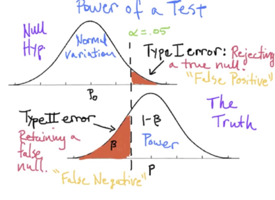
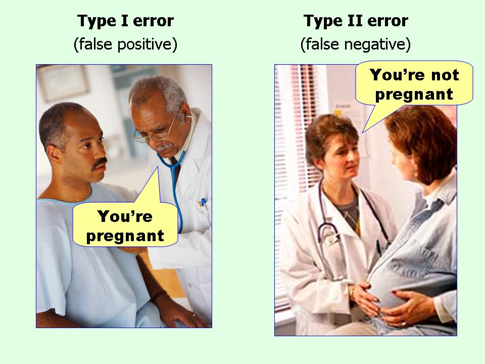
- Type 1 Error (AKA alpha error, or false positive error). This is when we falsely accept the alternative hypothesis, when the null hypothesis is true. For example, we find a difference in happiness score when there is no true difference. Note the – is the probability that a result is a result of chance, while the alpha level is the accepted false positive rate and is set a priori to the study.
- Type 2 error (AKA Beta error, or false negative error). This is when we falsely accept the null hypothesis that no difference exists when there actually is a difference. Eg we find no difference in happiness scores when there is one after all. The beta is the false negative rate minus the probability a true difference will be missed when one exists.
Q8. What does this P-value mean?
Medicine is subject to harms of error in both false positive (the alpha level) and false negative (the beta level) directions.
The alpha is usually set at <0.05.
Why?… Scientists are often trying to prove a difference, so avoiding over enthusiasm is important. Incorrectly proving a new intervention is effective may have far reaching consequences for patients, and it is important to first do no harm.
The Beta (or false negative rate) is usually set at a higher rate of 20%.
Why?… It is considered more acceptable to miss a true difference 20% of the time. This is because further studies should eventually show this important difference and it will be adopted at a later time. But the downside is that we may false reject important treatments, and deny patients to potential benefits of these treatments.
Note: Power is 1-Beta or 1-0.2 = 80%.
You want to calculate your sample size.
Q9. How many people will you need in your study?
(Hint – you already have your alpha and beta values above. You estimate a reasonable effect size to be 5 % points difference in happiness score. The standard deviation of the data is 6.)
To calculate sample size you need 4 pieces of information.
- Alpha level = 0.05
- Beta level = 0.8
- Effect size = 5 points (estimated from the observational study – the difference in values between study and controls groups)
- Standard deviation = 6 (Also estimated from the pilot studies)
Using the powerandsamplesize.com online calculator, the calculated sample size is 24.
Q10. List 4 factors which increase the required sample size?
- Increased variance of the data
- Small effect size
- Smaller alpha value
- Large Beta value
You complete your randomised controlled trial (RCT) and present the results to your friend. You don’t find any statistical relationship between coffee consumption and happiness in doctors. Thus your RCT doesn’t support your hypothesis, despite the promising observational data. You begin to slip into a nihilisitic ICU research fugue state… another “negative” trial… However your friend says you have now come of age as an critical care researcher and a dazzling future as a member of the ANZICS CTG no doubt awaits you!
References and links
- Nickson CP. Confidence Intervals. Critical Care Compendium, Lifeinthefastlane.com. 26 August 2015 [Accessed 30 October 2017] Available from: https://lifeinthefastlane.com/ccc/confidence-intervals/
- Nickson CP. Error in Research. Critical Care Compendium, Lifeinthefastlane.com. 26 August 2015 [Accessed 30 October 2017] Available from: https://lifeinthefastlane.com/ccc/error-in-research/
- Nickson CP. Power and Sample Size Calculation. Critical Care Compendium, Lifeinthefastlane.com. 26 August 2015 [Accessed 30 October 2017] Available from: https://lifeinthefastlane.com/ccc/power-and-sample-size-calculation/
- Nickson CP. Quantitative Data Types and Tests. Critical Care Compendium, Lifeinthefastlane.com. 26 August 2015 [Accessed 30 October 2017] Available from: https://lifeinthefastlane.com/ccc/quantitative-data-types-and-tests/
- Wasserstein RL, Lazar NA. The ASA’s Statement on -Values: Context, Process, and Purpose The American Statistician. 2016; 70(2):129-133. [article]
